Affinity plot
The affinity plot shows the relation between the association (ka) and dissociation (kd) rate constants and the equilibrium dissociation constant (KD).
The association rate constants are on the y-axis in red. The dissociation rate constants are in blue on the x-axis. The intersections of the ka and kd are the equilibrium dissociation constant in green. The green lines connect the points with the same KD. The intermediate yellow box marks the range in which most of the association and dissociation rate constants can be expected. The four red dots show examples of the curves at the intersections (the analyte concentration is 1 nM = 1 x KD).
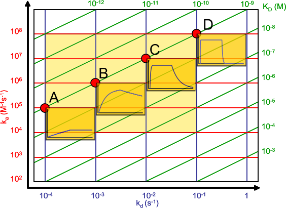
The affinity plot shows that the same equilibrium dissociation constant can have many different sensorgram shapes which depend on the rate constants. In addition the shape of the association curve is also dependent on the analyte concentration.
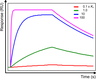
Compare the figure below with sensorgram B in the affinity plot. When the analyte concentration = 1x KD the curves look the same (scale is different). When the analyte concentration changes the association part changes but the dissociation part stays the same although due to the higher starting point the dissociation rate starts faster.
Time to equilibrium
An important experimental consideration is the time taken to reach equilibrium. From the integrated rate equation for association, the time required (tΘ) to reach a fraction of equilibrium (Θ= R/Req) can be derived as:

To reach steady state faster it is possible to raise the analyte concentration, but this will not always work. Analyte concentrations above 100 times KD often lead to binding curves that are not an exponential and the bulk shift disturbs the curve significantly. It is better to increase the injection time. However, as shown in the table below, this can take a very long. The time to reach steady state mainly depends on the dissociation rate constant. Long injection times are not always feasible due to the limited amount of sample or the maximal injection volume.
| concentration analyte | kd (s-1) | ||||
|---|---|---|---|---|---|
| 10-1 | 10-2 | 10-3 | 10-4 | ||
| 0.01 x KD | 68 s | 11.5 min | 115 min | 1140 min | |
| 0.1 x KD | 63 s | 10.5 min | 105 min | 1047 min | |
| 1 x KD | 34 s | 5.8 min | 57 min | 576 min | |
| 10 x KD | 6 s | 1 min | 10.5 min | 1105 min | |
| 100 x KD | 1 s | 0.1 min | 1 min | 11 min | |
| ka = 1.105 M-1s-1 | |||||